
List of Example Simulations
Sym8.EQ: Equilibrium Speciation, Seawater
Input
| Setup | Quantity (mol/kg) |
|---|---|
| Na | 0.47 |
| Cl | 0.55 |
| C | 0.002 |
| Ca | 0.011 |
| Mg | 0.053 |
| K | 0.01 |
| S | 0.029 |
| Si | 0.00015 |
| pH | 8.2 |
| T (°C) | 25 |
Output
| solute | concn (mol/kg) |
|---|---|
| CO2(aq) | 4.33047e-06 |
| CO3-- | 0.000428181 |
| Ca++ | 0.0109078 |
| CaCO3(aq) | 4.44815e-06 |
| CaCl+ | 6.39229e-05 |
| CaCl2(aq) | 2.48119e-06 |
| CaHCO3+ | 3.94987e-06 |
| CaHSiO3+ | 3.22952e-08 |
| CaOH+ | 2.65951e-08 |
| CaSO4(aq) | 1.7356e-05 |
| Cl- | 0.542727 |
| H+ | 7.94328e-09 |
| H2SO4(aq) | 5.61564e-22 |
| HCO3- | 0.00153571 |
| HSO4- | 4.40433e-10 |
| HSiO3- | 1.36603e-05 |
| K+ | 0.00995358 |
| KCl(aq) | 2.52684e-06 |
| KHSO4(aq) | 2.36038e-16 |
| KOH(aq) | 4.56413e-09 |
| KSO4- | 4.38891e-05 |
| Mg++ | 0.0524186 |
| Mg4(OH)4++++ | 1.59258e-11 |
| MgCO3(aq) | 9.58805e-06 |
| MgCl+ | 0.000441576 |
| MgHCO3+ | 1.85068e-05 |
| MgHSiO3+ | 2.75919e-07 |
| MgOH+ | 1.80852e-06 |
| MgSO4(aq) | 0.000109622 |
| Na+ | 0.464366 |
| NaCO3- | 1.37617e-05 |
| NaCl(aq) | 0.00676027 |
| NaHCO3(aq) | 0.000163227 |
| NaHSiO3(aq) | 6.89991e-05 |
| NaOH(aq) | 3.64901e-07 |
| NaSO4- | 0.00135406 |
| OH- | 7.93255e-06 |
| SO4-- | 0.0274751 |
| SiO2(aq) | 6.70324e-05 |
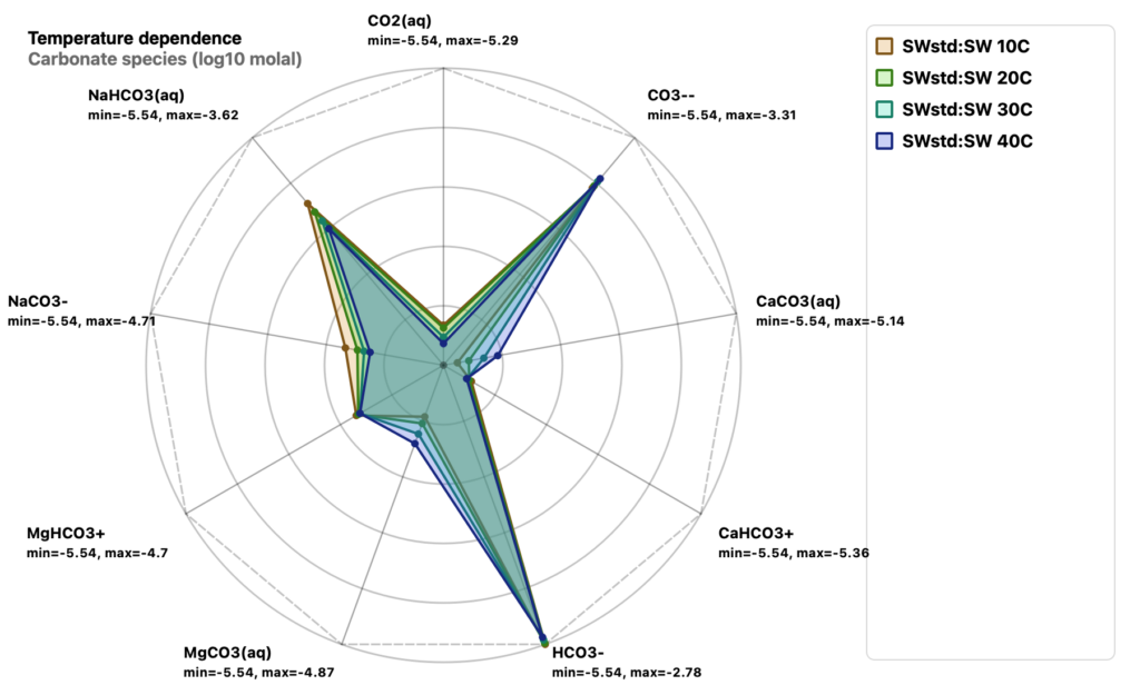
Carbonate species at different temperatures
Sym8.EQ: Fe and Mn Redox Pairs
Most natural groundwater systems are not in redox equilibrium. Fe²⁺/Fe³⁺, Mn²⁺/Mn³⁺, sulfate/sulfide, and many other redox couples commonly coexist at different implied redox potentials because of kinetic limitations, microbial activity, and transport processes. Yet many geochemical simulators describe the entire system using a single redox condition, masking important details of the interactions among different redox couples.
Sym8 removes the distinction between redox reactions and every other equilibrium reaction. There is no special redox basis species and no master redox variable around which the system pivots. Sym8 treats redox reactions in the same mathematical framework as other chemical reactions, without requiring a special redox basis species or master redox variable.
This framework also allows individual redox couples to remain in disequilibrium by directly constraining measured solute ratios. This is possible because Sym8 defines chemical composition through elemental mass conservation rather than through a basis-species formulation. Without a designated redox basis species, individual redox couples can be treated as ordinary equilibrium reactions while remaining independently constrained.
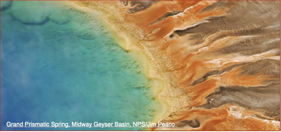
The color zonation reflects both temperature-driven redox gradients and microbial kinetic control. The
orange and red outer bands are where Fe and Mn chemistry becomes dominant. The inner blue area is
abiotic and reducing; green/yellow area is the transitional redox zone; and orange/brown outer rim is
dominated by Fe/Mn oxidation, either abiotic or microbial mediated.
Sym8.EQ allows flexible modes of redox speciation modeling without the use of kinetics. All redox couples can be constrained to equilibrium at a specified Eh. Or, selected redox couples can be constrained by measured solute ratios (for example, Fe²⁺/Fe³⁺ or Mn²⁺/Mn³⁺), while other couples remain at equilibrium. This flexibility make it possible to simulate chemically consistent solutions spanning a range of redox disequilibrium states.
To explore this behavior, I ran a series of aqueous speciation calculations over Eh values from −0.2 to +0.5 V while independently varying the Fe²⁺/Fe³⁺ and Mn²⁺/Mn³⁺ activity ratios. Total dissolved Fe and Mn were held constant within each simulation series.
| Composition (mol/kg) | |
|---|---|
| Fe | 0.001 |
| Mn | 5E-05 |
| Mg | 1E-04 |
| Ca | 1E-04 |
| K | 1E-04 |
| Na | < 0.005 |
| HCO3- | 0.001 |
| S | 0.001 |
| pH | 7 |
| Eh | -0.2 to 0.5 V |
| Redox Solutes | log10 (Ratio) |
| Fe++/Fe+++ | -6 to 2 |
| Mn++/Mn+++ | -8 to 8 |
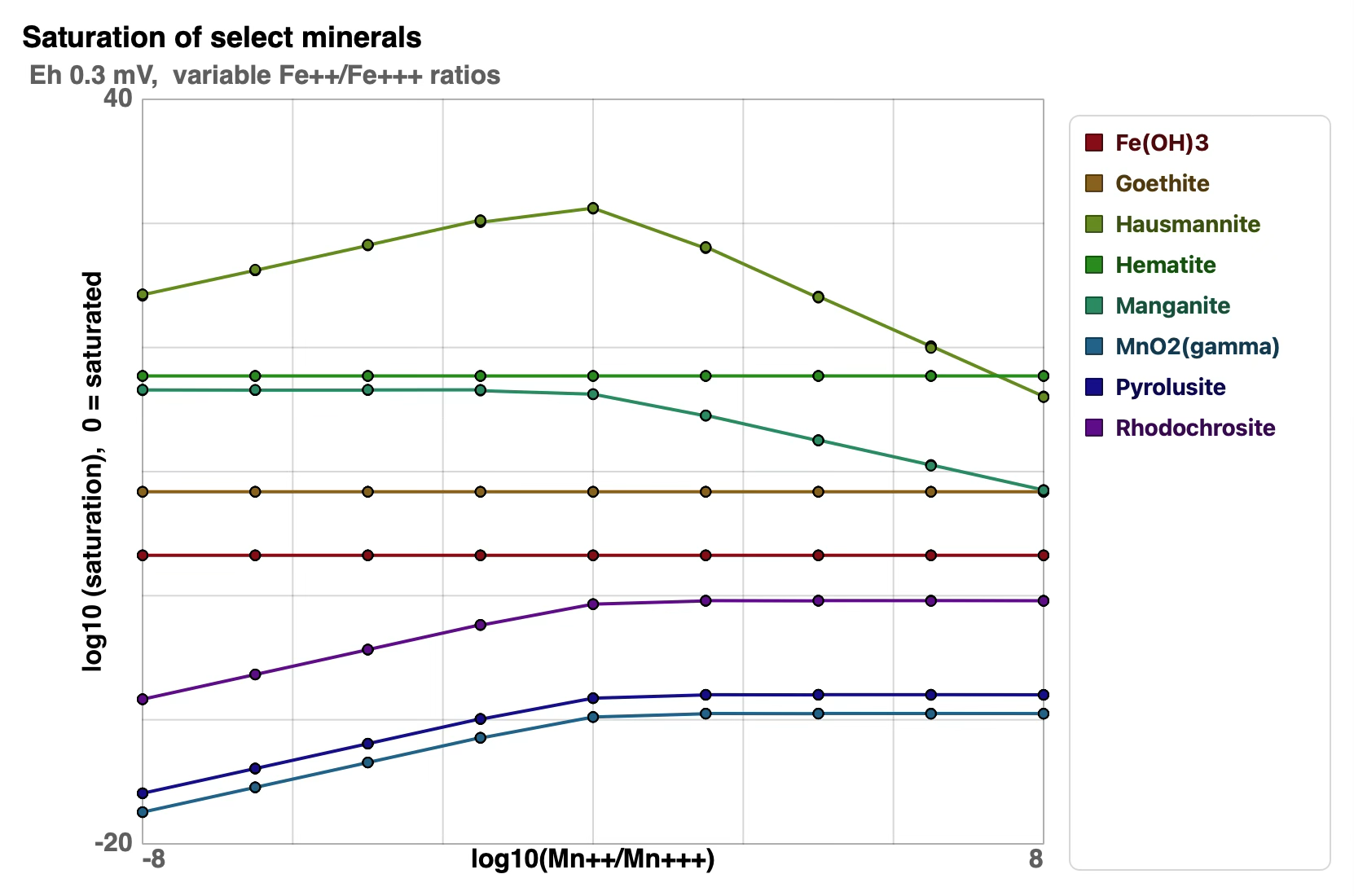
Saturations of selected minerals from simulations at fixed Eh = 0.3 V
and varying Fe²⁺/Fe³⁺ and Mn²⁺/Mn³⁺ ratios are shown. For the minerals
included in this plot, saturation does not vary with Fe²⁺/Fe³⁺. Fe-bearing
minerals are also independent of Mn²⁺/Mn³⁺, while Mn-bearing mineral
trends reflect changes in the relative abundances of Mn²⁺ and Mn³⁺. The
table at right shows the elemental composition used for all simulations.
The resulting mineral saturation patterns reveal a striking difference between the Fe and Mn systems.
Under the conditions illustrated here, free Fe²⁺ and Fe³⁺ account for only a small fraction of dissolved Fe, while Fe(OH)₂⁺ and Fe(OH)₃(aq) dominate the aqueous Fe inventory. As the imposed Fe²⁺/Fe³⁺ ratio changes, Fe³⁺ remains nearly constant while Fe²⁺ changes strongly. Consequently, Fe(III) minerals such as hematite and goethite show little change in saturation, while Fe(II)-bearing siderite and mixed-valence magnetite respond to the changing Fe ratio.
The Mn system behaves quite differently. Mn²⁺ and Mn³⁺ are the dominant dissolved Mn species, so changing the Mn²⁺/Mn³⁺ ratio directly redistributes a substantial portion of the dissolved Mn inventory. The resulting changes in saturation are correspondingly much larger and vary considerably among Mn minerals.
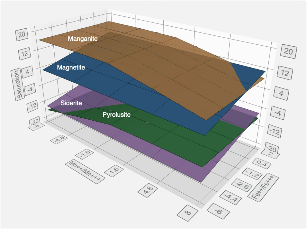
The 3D saturation surfaces illustrate another aspect of the results. Mn minerals respond strongly along the Mn²⁺/Mn³⁺ axis but are essentially independent of the Fe²⁺/Fe³⁺ ratio. Fe minerals show the complementary behavior: siderite and magnetite respond to the Fe ratio while remaining essentially independent of the Mn ratio.
These results illustrate an important consequence of redox disequilibrium: mineral response depends not simply on the imposed redox ratio, but on how the redox-pair species participate in the overall aqueous speciation.
Saturation surfaces of selected minerals from the same simulations shown in the scatter plot are presented here, illustrating the response of Mn- and Fe-bearing minerals to variable redox-solute distributions. Magnetite, containing both Fe(II) and Fe(III), and siderite, containing Fe(II), show changing saturation trends with varying Fe²⁺/Fe³⁺ ratio, while the Mn-bearing minerals respond primarily to changes in Mn²⁺/Mn³⁺. Changing the solution Eh (not shown) further shifts these saturation surfaces upward or downward, with the magnitude of the shift differing among minerals.
Sym8.BK: Mediterranean Salt Flat Evaporation
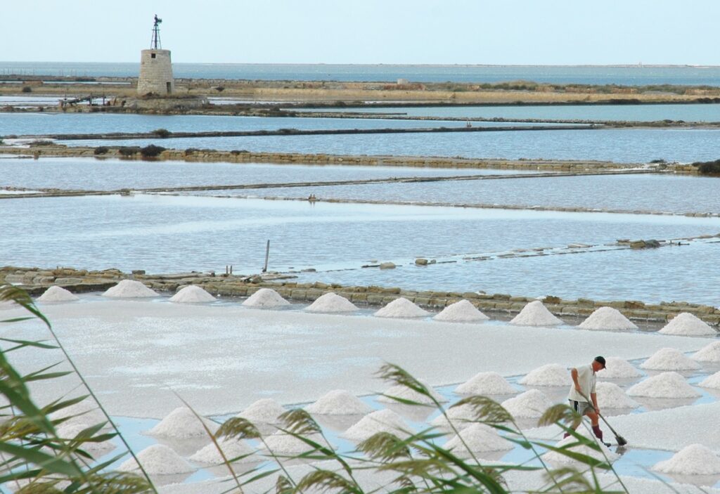
Evaporation of representative Mediterranean seawater is modeled using documented seasonal temperature and evaporation-rate trends. Simulation results are compared with observed salt-flat mineralization patterns. The simulation begins in April with a 1-meter water column, equivalent to 103 g of water (water mass density of 1.03 g for each cc).
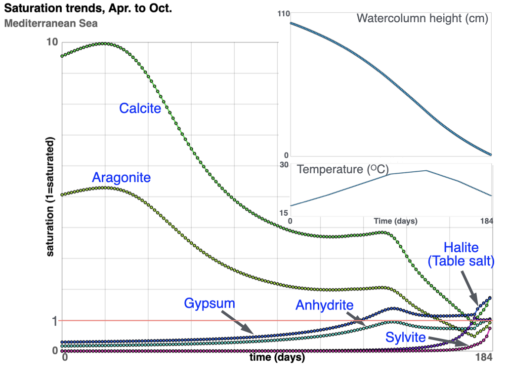
The model tracks progressive evaporation of water together with kinetic reactions involving dissolved salts and minerals. Halite (table salt) begins to precipitate after approximately 95% of the original water volume has evaporated. In contrast, anhydrite, calcite, and aragonite become thermodynamically favorable much earlier in the evaporation sequence; however, because of their relatively slow kinetic reaction rates, only minor amounts precipitate by the end of the simulation.
photo: Saline di Trapani, Sicilia, by Click.gianluca - Own work, CC BY-SA 4.0, Link

Simulation condition
| month | ° C | evap. mm/day |
|---|---|---|
| Apr. | 18 | 3 |
| May | 21 | 4 |
| June | 24 | 5.5 |
| July | 27 | 7 |
| Aug. | 28 | 7.5 |
| Sept. | 25 | 5.5 |
| Oct. | 21 | 4 |
Starting water
| solute | mol/kg |
|---|---|
| Na+ | 0.49 |
| Cl- | 0.57 |
| Mg++ | 0.054 |
| SO4-- | 0.029 |
| Ca++ | 0.011 |
| K+ | 0.01 |
| pH | 8.1 |
| alkalinity | 0.0025 |
saturation trends during evaporation
Comparison (volume, cc)
| salt | observed | simulated |
|---|---|---|
| Halite (table salt) | 1.2 - 1.4 | 1.2 |
| Gypsum / Anhydrite | 0.1 - 0.3 | 0.1 |
| Carbonate | minor | < 2e-7 |
| Sylvite | minor | < 1e-7 |
The change in sulfate and carbonate saturation trends near the five-month point corresponds to the onset of gypsum precipitation. Gypsum saturation initially rises above equilibrium because dissolved ion concentrations increase faster than gypsum crystals can nucleate and grow. As gypsum precipitation progresses, crystal growth increases the available reactive surface area, allowing precipitation rates to accelerate and eventually keep pace with the continuing concentration of dissolved solutes. This causes the saturation curve to stabilize and subsequently decline.
Sym8.BK: Chromium Removal from Wastewater
Treatment ponds are widely used to remove dissolved metals and contaminants from industrial and mining wastewater through natural chemical and mineral reactions. This example uses Sym8.BK to model chromium removal in a passive treatment pond under continuously changing chemical and environmental conditions.
Chromium removal in treatment ponds commonly occurs through adsorption onto reactive iron oxyhydroxide precipitates and through precipitation of chromium-bearing mineral phases. As water chemistry evolves through evaporation, oxidation, pH adjustment, and mineral reactions, dissolved chromium concentrations can decrease substantially over time.
In this example, the reaction between iron oxyhydroxide and dissolved chromium-bearing species to form Cr-bearing ferrihydrite is modeled. Reactive iron oxyhydroxide acts as a reducing and adsorbing agent that promotes the conversion of dissolved Cr(VI), which is highly mobile in water, to the less soluble Cr(III) oxidation state. The resulting Cr(III)-rich precipitates become incorporated into iron oxyhydroxide mineral phases, allowing chromium to be removed and recovered from the wastewater system.
Speciation of Chrome (Cr) and Iron (Fe)
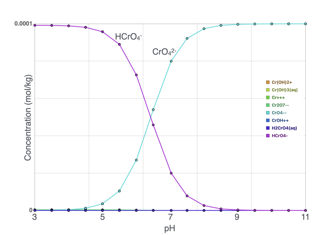
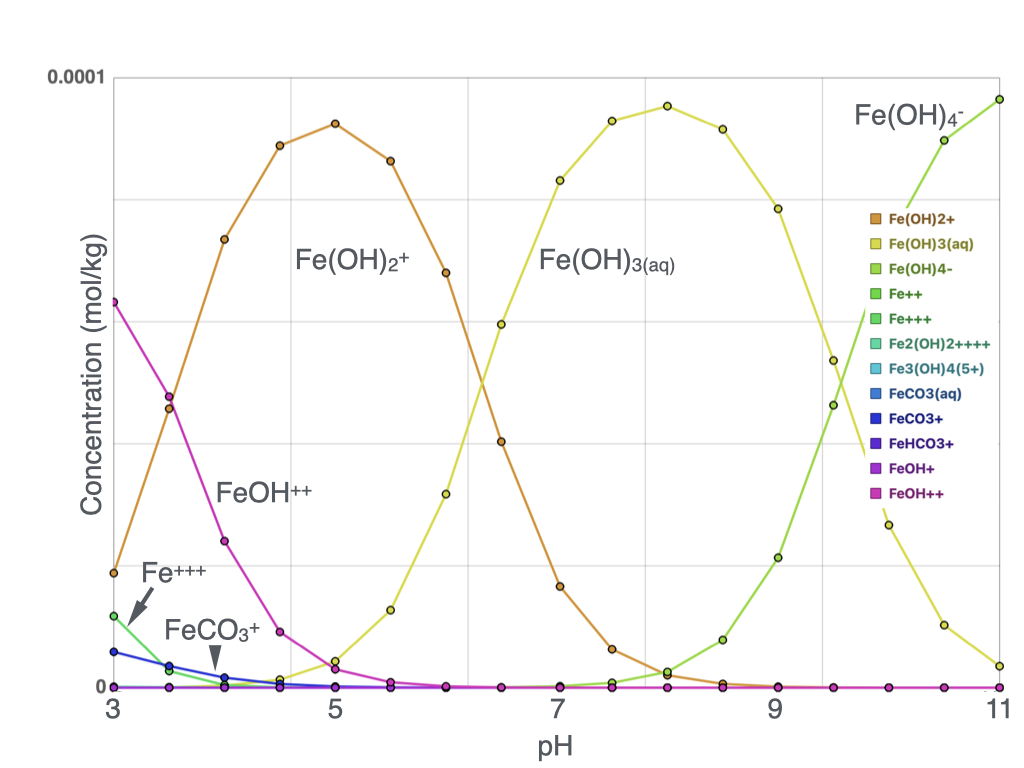
In a redox reaction, electrons are transferred between chemical species. In this simulation, Cr(VI) acts as the electron acceptor and becomes reduced, while Fe(II) acts as the electron donor and becomes oxidized. The reaction produces less soluble Fe–Cr mineral phases that precipitate from the water and stabilize chromium.
Chromium Stabilization: pH, Redox, and Fe-Cr Mineral Precipitation
| rate constant | 1.0e-8 | volume | 1 liter (1 kg) |
|---|---|---|---|
| Fe(OH)3 | 0.5 cc (1.8 g) | T | 25 ° C |
| Cr(OH)3(am) | 0.2 cc (0.7 g) | Na2CO3 | 0.3 - 1.3 cc (0.8 - 3.3 g) |
| Simulation duration: 1 day | |||
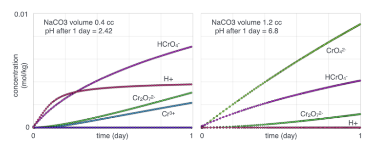
Formation of this precipitate requires dissolution of Fe(OH)₃ to supply dissolved iron. Dissolution of Fe(OH)₃ and Cr(OH)₃(am) tends to acidify the solution, which can increase dissolved chromium concentrations and reduce precipitation efficiency.
To maintain neutral to alkaline conditions, varying amounts of Na₂CO₃ are added. The figure on the left represents conditions with little or no Na₂CO₃ addition, whereas the figure on the right represents conditions with Na₂CO₃ added in excess relative to Cr(OH)₃(am). Under neutral to alkaline conditions, CrO₄²⁻ becomes the dominant dissolved chromium species, and precipitation of Cr–Fe hydroxide phases is enhanced.
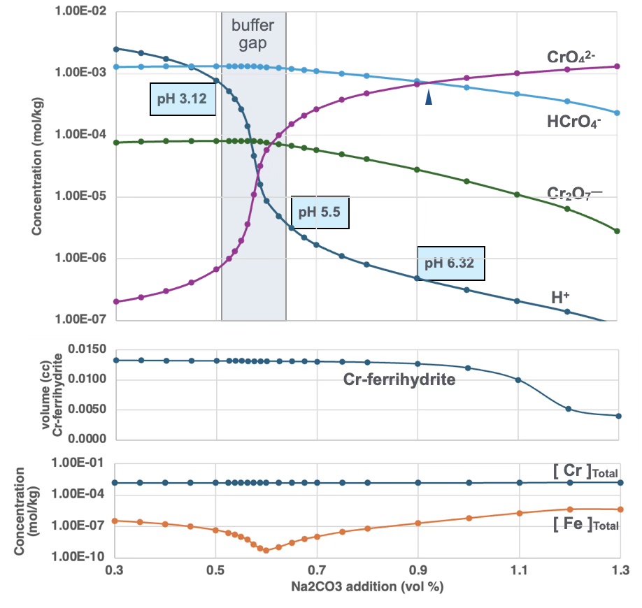
The second plot shows total volume of Cr-ferrihydrite precipitated; the third plot shows total Cr and Fe dissolved in water. Ferrihydrite volume is relatively consistent across the pH range, peaking near neutral conditions. Total dissolved Cr is similarly consistent across the pH range. Total Fe in solution increases toward higher pH, but Fe³⁺ concentration — the species controlling ferrihydrite precipitation — decreases with increasing pH, becoming the limiting factor for Cr removal under alkaline conditions.
The buffering gap observed between approximately pH 3 and 5 results from complex interactions among dissolved species and proton balance. Within this region, small changes in Na₂CO₃ addition produce relatively large changes in solution pH. This transition zone also coincides with a rapid increase in dissolved CrO₄²⁻ concentration; however, the crossover point at which CrO₄²⁻ becomes more abundant than HCrO₄⁻ occurs at approximately pH 6.5.
The quantity of Cr-bearing ferrihydrite precipitated also varies with pH. At elevated pH, little to no Cr–ferrihydrite precipitates despite increasing CrO₄²⁻ concentration, because dissolved Fe³⁺ concentration decreases more strongly and becomes the limiting factor for precipitation. Under acidic conditions, greater quantities of dissolved chromium remain in solution, which is not favorable for chromium removal. The most effective chromium removal in this simulation occurs under near-neutral pH conditions, where dissolved chromium concentrations are minimized while precipitation of chromium-bearing ferrihydrite is maximized.
Sym8.BK: Chromium Removal - Passive Wastewater Treatment Pond
More Contents Coming Soon
Sym8.BK: Ostwald Step Rule - Silica Transformation Sequence
The Ostwald step rule describes a process in which minerals of the same chemical composition transform through a sequence of progressively more stable phases over time. Unlike Ostwald ripening, which involves grain-size-driven competition between small and large crystals, the Ostwald step rule is controlled by differences in thermodynamic stability and reaction kinetics between mineral phases.
One of the best-known geological examples is the recrystallization sequence of silica polymorphs involving opal-A, opal-CT, and quartz. In silica-supersaturated waters, opal-A commonly precipitates first as the least ordered and most metastable phase. Over time, it gradually dissolves and recrystallizes into opal-CT, which eventually transforms into the more stable quartz phase.
Agate is a textbook natural expression of Ostwald's step rule: silica precipitated from aqueous solution begins as amorphous SiO₂ or silica gel, ripens through opal-A and opal-CT, organizes into fibrous chalcedony, and finally crystallizes as macrocrystalline quartz toward the center of the nodule. The banded rim-to-core progression preserved in a single slice is, in effect, Ostwald's rule frozen in stone.
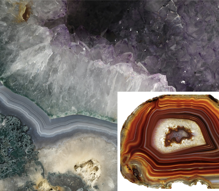
photo: Katriona McCarthy on Unsplash; inset photo: gemstonebuzz.com
Simulation Setup
| temperature | 70 °C |
|---|---|
| total duration | 2.5 years |
| starting volume of SiO2(am) | 20 cc |
| starting grain size of SiO2(am) | 0.004 mm |
| rate constant and nucleation threshhold | moles/ cm^2-sec, Q/K |
| SiO2(am) | 1.0e-9, 1.1 |
| chalcedony | 1.0e-10, 1.5 |
| quartz | 1.0e-11, 2.0 |
| performance | |
| cpu time | 1 minute |
| total timesteps | 130,000 |
Silica Growth Pattern
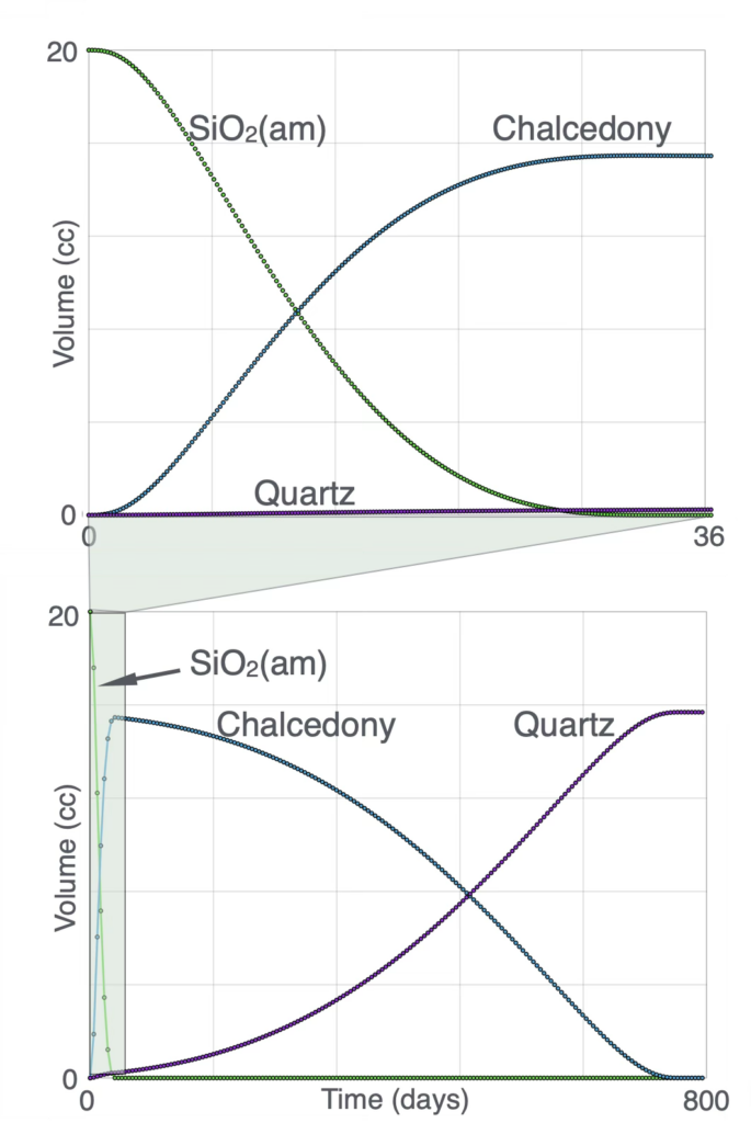
During the first 30 days quartz precipitation begins while the SiO₂(am)-to-chalcedony transformation is still occurring because the rapid dissolution of SiO₂(am) causes dissolved silica concentrations to exceed the saturation limits of both chalcedony and quartz.
Although the kinetic reaction rates of the three silica phases differ by approximately one order of magnitude, their thermodynamic stabilities differ much more significantly, resulting in a substantially longer time required to convert chalcedony to quartz than to convert SiO₂(am) to chalcedony.
Variations in the initial quantity and grain size of SiO₂(am), as well as changes in temperature, can alter the transformation rates and timing; however, the overall sequence of silica phase transformation remains the same.