Sym8.EQ Equilibrium Speciation: Seawater
Input
| Setup | Quantity (mol/kg) |
|---|---|
| Na | 0.47 |
| Cl | 0.55 |
| C | 0.002 |
| Ca | 0.011 |
| Mg | 0.053 |
| K | 0.01 |
| S | 0.029 |
| Si | 0.00015 |
| pH | 8.2 |
| T (°C) | 25 |
Output
| solute | concn (mol/kg) |
|---|---|
| CO2(aq) | 4.33047e-06 |
| CO3-- | 0.000428181 |
| Ca++ | 0.0109078 |
| CaCO3(aq) | 4.44815e-06 |
| CaCl+ | 6.39229e-05 |
| CaCl2(aq) | 2.48119e-06 |
| CaHCO3+ | 3.94987e-06 |
| CaHSiO3+ | 3.22952e-08 |
| CaOH+ | 2.65951e-08 |
| CaSO4(aq) | 1.7356e-05 |
| Cl- | 0.542727 |
| H+ | 7.94328e-09 |
| H2SO4(aq) | 5.61564e-22 |
| HCO3- | 0.00153571 |
| HSO4- | 4.40433e-10 |
| HSiO3- | 1.36603e-05 |
| K+ | 0.00995358 |
| KCl(aq) | 2.52684e-06 |
| KHSO4(aq) | 2.36038e-16 |
| KOH(aq) | 4.56413e-09 |
| KSO4- | 4.38891e-05 |
| Mg++ | 0.0524186 |
| Mg4(OH)4++++ | 1.59258e-11 |
| MgCO3(aq) | 9.58805e-06 |
| MgCl+ | 0.000441576 |
| MgHCO3+ | 1.85068e-05 |
| MgHSiO3+ | 2.75919e-07 |
| MgOH+ | 1.80852e-06 |
| MgSO4(aq) | 0.000109622 |
| Na+ | 0.464366 |
| NaCO3- | 1.37617e-05 |
| NaCl(aq) | 0.00676027 |
| NaHCO3(aq) | 0.000163227 |
| NaHSiO3(aq) | 6.89991e-05 |
| NaOH(aq) | 3.64901e-07 |
| NaSO4- | 0.00135406 |
| OH- | 7.93255e-06 |
| SO4-- | 0.0274751 |
| SiO2(aq) | 6.70324e-05 |
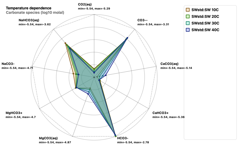
Carbonate species at different temperatures
Sym8.BK Reactive-Kinetic Simulation:
Mediterranean Salt Flat Evaporation Model
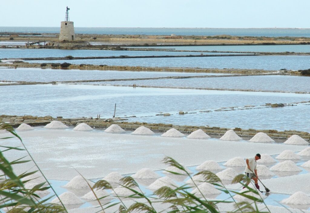
Evaporation of representative Mediterranean seawater is modeled using documented seasonal temperature and evaporation-rate trends. Simulation results are compared with observed salt-flat mineralization patterns. The simulation begins in April with a 1-meter water column, equivalent to 103 g of water (water mass density of 1.03 g for each cc).
The model tracks progressive evaporation of water together with kinetic reactions involving dissolved salts and minerals. Halite (table salt) begins to precipitate after approximately 95% of the original water volume has evaporated. In contrast, anhydrite, calcite, and aragonite become thermodynamically favorable much earlier in the evaporation sequence; however, because of their relatively slow kinetic reaction rates, only minor amounts precipitate by the end of the simulation.
photo: Saline di Trapani, Sicilia, by Click.gianluca - Own work, CC BY-SA 4.0, Link
Simulation condition
| month | ° C | evap. mm/day |
|---|---|---|
| Apr. | 18 | 3 |
| May | 21 | 4 |
| June | 24 | 5.5 |
| July | 27 | 7 |
| Aug. | 28 | 7.5 |
| Sept. | 25 | 5.5 |
| Oct. | 21 | 4 |
Starting water
| solute | mol/kg |
|---|---|
| Na+ | 0.49 |
| Cl- | 0.57 |
| Mg++ | 0.054 |
| SO4-- | 0.029 |
| Ca++ | 0.011 |
| K+ | 0.01 |
| pH | 8.1 |
| alkalinity | 0.0025 |
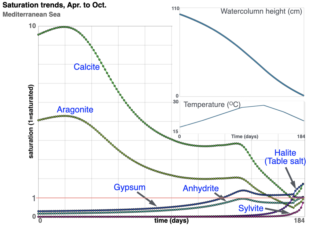
saturation trends during evaporation
Comparison (volume, cc)
| salt | observed | simulated |
|---|---|---|
| Halite (table salt) | 1.2 - 1.4 | 1.2 |
| Gypsum / Anhydrite | 0.1 - 0.3 | 0.1 |
| Carbonate | minor | < 2e-7 |
| Sylvite | minor | < 1e-7 |
The change in sulfate and carbonate saturation trends near the five-month point corresponds to the onset of gypsum precipitation. Gypsum saturation initially rises above equilibrium because dissolved ion concentrations increase faster than gypsum crystals can nucleate and grow. As gypsum precipitation progresses, crystal growth increases the available reactive surface area, allowing precipitation rates to accelerate and eventually keep pace with the continuing concentration of dissolved solutes. This causes the saturation curve to stabilize and subsequently decline.
Chromium Removal from Wastewater
Treatment ponds are widely used to remove dissolved metals and contaminants from industrial and mining wastewater through natural chemical and mineral reactions. This example uses Sym8.BK to model chromium removal in a passive treatment pond under continuously changing chemical and environmental conditions.
Chromium removal in treatment ponds commonly occurs through adsorption onto reactive iron oxyhydroxide precipitates and through precipitation of chromium-bearing mineral phases. As water chemistry evolves through evaporation, oxidation, pH adjustment, and mineral reactions, dissolved chromium concentrations can decrease substantially over time.
In this example, the reaction between iron oxyhydroxide and dissolved chromium-bearing species to form Cr-bearing ferrihydrite is modeled. Reactive iron oxyhydroxide acts as a reducing and adsorbing agent that promotes the conversion of dissolved Cr(VI), which is highly mobile in water, to the less soluble Cr(III) oxidation state. The resulting Cr(III)-rich precipitates become incorporated into iron oxyhydroxide mineral phases, allowing chromium to be removed and recovered from the wastewater system.
Speciation of Chrome (Cr) and Iron (Fe)
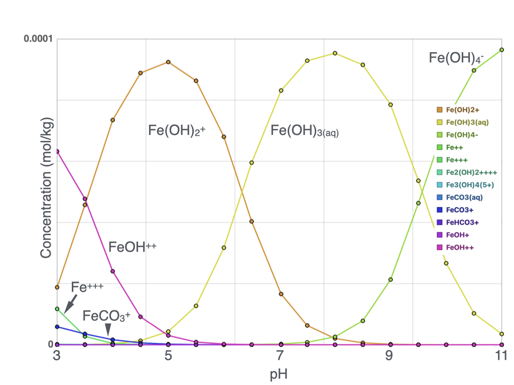
In a redox reaction, electrons are transferred between chemical species. In this simulation, Cr(VI) acts as the electron acceptor and becomes reduced, while Fe(II) acts as the electron donor and becomes oxidized. The reaction produces less soluble Fe–Cr mineral phases that precipitate from the water and stabilize chromium.
Chromium Stabilization: pH, Redox, and Fe-Cr Mineral Precipitation
| rate constant | 1.0e-8 | volume | 1 liter (1 kg) |
|---|---|---|---|
| Fe(OH)3 | 0.5 cc (1.8 g) | T | 25 ° C |
| Cr(OH)3(am) | 0.2 cc (0.7 g) | Na2CO3 | 0.3 - 1.3 cc (0.8 - 3.3 g) |
| Simulation duration: 1 day | |||
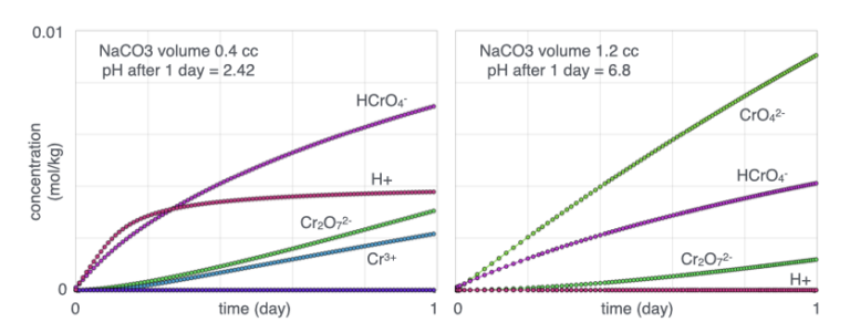
Formation of this precipitate requires dissolution of Fe(OH)₃ to supply dissolved iron. Dissolution of Fe(OH)₃ and Cr(OH)₃(am) tends to acidify the solution, which can increase dissolved chromium concentrations and reduce precipitation efficiency.
To maintain neutral to alkaline conditions, varying amounts of Na₂CO₃ are added. The figure on the left represents conditions with little or no Na₂CO₃ addition, whereas the figure on the right represents conditions with Na₂CO₃ added in excess relative to Cr(OH)₃(am). Under neutral to alkaline conditions, CrO₄²⁻ becomes the dominant dissolved chromium species, and precipitation of Cr–Fe hydroxide phases is enhanced.
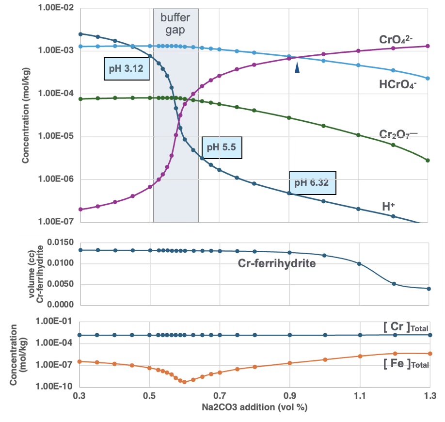
The second plot shows total volume of Cr-ferrihydrite precipitated; the third plot shows total Cr and Fe dissolved in water. Ferrihydrite volume is relatively consistent across the pH range, peaking near neutral conditions. Total dissolved Cr is similarly consistent across the pH range. Total Fe in solution increases toward higher pH, but Fe³⁺ concentration — the species controlling ferrihydrite precipitation — decreases with increasing pH, becoming the limiting factor for Cr removal under alkaline conditions.
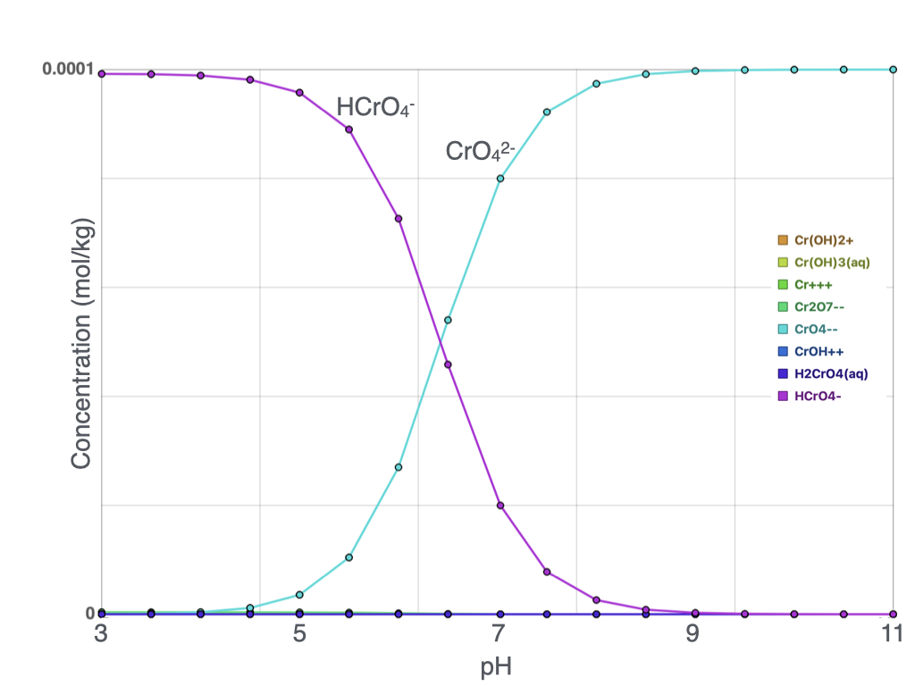
The buffering gap observed between approximately pH 3 and 5 results from complex interactions among dissolved species and proton balance. Within this region, small changes in Na₂CO₃ addition produce relatively large changes in solution pH. This transition zone also coincides with a rapid increase in dissolved CrO₄²⁻ concentration; however, the crossover point at which CrO₄²⁻ becomes more abundant than HCrO₄⁻ occurs at approximately pH 6.5.
The quantity of Cr-bearing ferrihydrite precipitated also varies with pH. At elevated pH, little to no Cr–ferrihydrite precipitates despite increasing CrO₄²⁻ concentration, because dissolved Fe³⁺ concentration decreases more strongly and becomes the limiting factor for precipitation. Under acidic conditions, greater quantities of dissolved chromium remain in solution, which is not favorable for chromium removal. The most effective chromium removal in this simulation occurs under near-neutral pH conditions, where dissolved chromium concentrations are minimized while precipitation of chromium-bearing ferrihydrite is maximized.
Chromium Removal: Passive Wastewater Treatment Pond
More Contents Coming Soon
Ostwald Step Rule: Silica Transformation Sequence
The Ostwald step rule describes a process in which minerals of the same chemical composition transform through a sequence of progressively more stable phases over time. Unlike Ostwald ripening, which involves grain-size-driven competition between small and large crystals, the Ostwald step rule is controlled by differences in thermodynamic stability and reaction kinetics between mineral phases.
One of the best-known geological examples is the recrystallization sequence of silica polymorphs involving opal-A, opal-CT, and quartz. In silica-supersaturated waters, opal-A commonly precipitates first as the least ordered and most metastable phase. Over time, it gradually dissolves and recrystallizes into opal-CT, which eventually transforms into the more stable quartz phase.
Agate is a textbook natural expression of Ostwald's step rule: silica precipitated from aqueous solution begins as amorphous SiO₂ or silica gel, ripens through opal-A and opal-CT, organizes into fibrous chalcedony, and finally crystallizes as macrocrystalline quartz toward the center of the nodule. The banded rim-to-core progression preserved in a single slice is, in effect, Ostwald's rule frozen in stone.
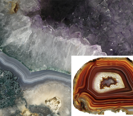
photo: Katriona McCarthy on Unsplash; inset photo: gemstonebuzz.com
Simulation setup
| temperature | 70 °C |
|---|---|
| total duration | 2.5 years |
| starting volume of SiO2(am) | 20 cc |
| starting grain size of SiO2(am) | 0.004 mm |
| rate constant and nucleation threshhold | moles/ cm^2-sec, Q/K |
| SiO2(am) | 1.0e-9, 1.1 |
| chalcedony | 1.0e-10, 1.5 |
| quartz | 1.0e-11, 2.0 |
| performance | |
| cpu time | 1 minute |
| total timesteps | 130,000 |
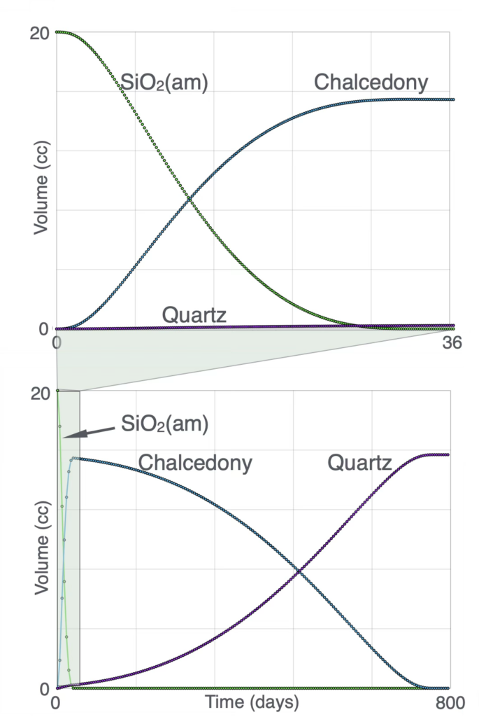
Silica Growth Pattern
During the first 30 days quartz precipitation begins while the SiO₂(am)-to-chalcedony transformation is still occurring because the rapid dissolution of SiO₂(am) causes dissolved silica concentrations to exceed the saturation limits of both chalcedony and quartz.
Although the kinetic reaction rates of the three silica phases differ by approximately one order of magnitude, their thermodynamic stabilities differ much more significantly, resulting in a substantially longer time required to convert chalcedony to quartz than to convert SiO₂(am) to chalcedony.
Variations in the initial quantity and grain size of SiO₂(am), as well as changes in temperature, can alter the transformation rates and timing; however, the overall sequence of silica phase transformation remains the same.